Forest Cover Type Prediction

Forest Cover Type Prediction

In this Kaggle competition [link], we are asked to predict forest cover type from strictly cartographic variables. (USFS). The data is in raw (unscaled) format and contains binary columns of data for qualitative independent variables, such as wilderness and soil type.

The study area includes four wilderness areas located in the Roosevelt National Forest of northern Colorado. Each observation is a 30m x 30m patch. You are asked to predict an integer classification for the forest cover type. The seven types are:

The training set (15120 observations) contains both features and the Cover_Type. The test set contains only the features. You must predict the Cover_Type for every row in the test set (565892 observations).

In this case I use a single notebook loadable from google colab.

First, the corresponding EDA is carried out. In this EDA, the great variability of the data comes to light from distance, grades, indices to categorical variables that represent the existence or not of different types of soils in the different Wilderness Areas (which also represent a variable). It can also be seen how the target variable is well distributed in the training data (2160 each).

Two types of univariate and bivariate analyzes are performed in the EDA.

Univariate Analysis resume:

• Train dataset has 15120 rows and 56 columns.
• There are no NA in the dataset. Therefore, the dataset is properly formatted and balanced.
• Each column has numeric (integer/float) datatype.
• Only 4 columns had outliers Horizontal_Distance_To_Hydrology, Vertical_Distance_To_Hydrology,
  Horizontal_Distance_To_Roadways and Horizontal_Distance_To_Fire_Points.
• Cover_Type is our label/target column.

Bivariate Analysis resume:

• The importance of the categorical variable Wilderness Area Type (created from the variables Wilderness_Area#) is verified by analyzing the density and distribution of the values with respect to the values of our target variable Cover_Type.
• Some high correlations between hillshade variables, distance to hydrology. Makes sense since these variables seem interrelated.
• The Relation and Distribution of continuous variables (Elevation, Aspect, Slope, Distance and Hillsahde columns) were analyzed in addition to the highly correlated features such as: (hillshade noon - hillshade 3pm),
  (hillshade 3 pm - hillshade 9 am), (vertical distance to hydrology - horizontal distance to hydrology) and (elevation - slope)
• The pearson coefficients showed that none of the base features have significantly linear effect in determining the label cover type. In addition, one interesting finding was that Soil Type 7 and 15 correlation are none in the pearson table, or what is the same it has no effect on determining the label Cover_Type according to the data.

Baseline Results (No Feature Engineering)

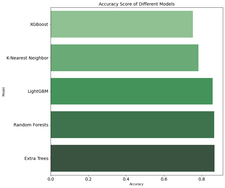
In this section, the results of different models would be analyzed with the features without Feature Engineering to select a model in the first instance.

Extreme (extra) random forests outperformed other algorithms with better accuracy performance in this case. The reason might be, I did not focus on tuning the parameters of the each algorithm and used defaults values instead. In any case, due to the type of problem that arises, we will focus on the feature engineering and hyperparameter tuning of a Extreme (extra) random forests.

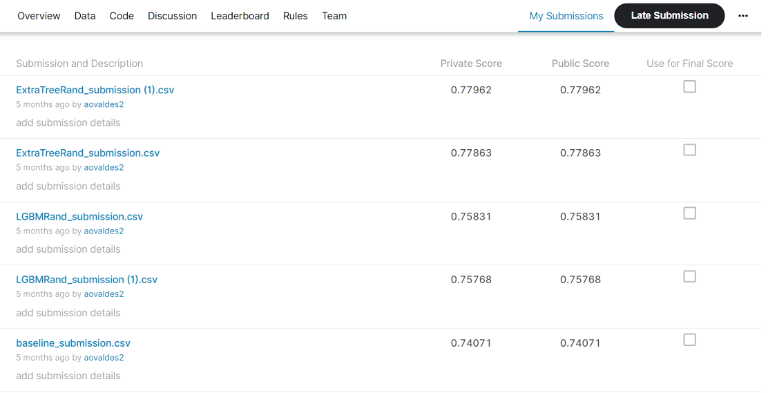
This baseline submision score 0.74071 in the Kaggle Competition.

Feature Engineering & Selection

Since the test data is much larger than the training data, and performs differently, I'm not going to remove any predictors. Instead I'm going to focus on creating new ones that highlight similarities in the data. Due to the characteristics of some features, it would make sense to introduce new ones and observe their implication in the models.

Feature engineering was separated into blocks to compare their improvement in the scores. Engineering was used from the simplest of adding columns or having maxima to some more complex ones such as adding absolutes or Euclidean distances to certain points, always based on the characteristics of the features themselves.

Adding a few at a time and then checked the results on the validation data we can see especially for the extra trees model, accuracy kept increasing as predictors were added.

Perform Hyperparameter Tuning on the Bests Models

As we know optimizing the hyperparameters for machine learning models is vital to the performance of the machine learning models and the process of tuning the HPs is not intuitive and can be a complex task. In this case its use Randomized Search for a shorter run-time although may not return the best combination of hyper-parameters that would return the best accuracy, this method doesn't consider past evaluations and it will continue the iterations regardless of the results. In the end, for the chosen model, it was obtained:

Best ExtraTreesClassifier Params: {'n_estimators': 300, 'min_samples_split': 2, 'min_samples_leaf': 1, 'max_features': None}
						

Also as part of the experimentation, the parameters of a Light Gradient Boosting Machine classifier model were tuned with the same predictors mentioned above:

Best LGBMClassifier Params: {'num_leaves': 31, 'n_estimators': 200, 'max_depth': 5, 'learning_rate': 0.6}
						

In the following image we can see the best submissions where it can be noted that in the entries written in the form Name(1) all the predictors were already included but as part of the experimentation in the first instance there were fewer created features.

• View Project Code